- CFA Exams
- 2026 Level II
- Topic 1. Quantitative Methods
- Learning Module 1. Basics of Multiple Regression and Underlying Assumptions
- Subject 3. Assumptions Underlying Multiple Linear Regression
Why should I choose AnalystNotes?
Simply put: AnalystNotes offers the best value and the best product available to help you pass your exams.
Subject 3. Assumptions Underlying Multiple Linear Regression PDF Download
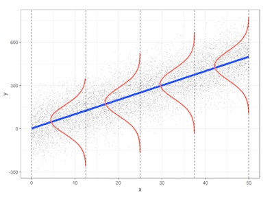
The assumptions of classical normal multiple linear regression model are as follows:
1. linearity. A linear relation exists between the dependent variable, Yt, and the independent variables (X1t, X2t, ..., Xkt).
2. Homoscedasticity. The variance of the error term is the same for all values of the independent variables.
3. Independence of Errors, or No Serial Correlation. The error term (et) is uncorrelated across observations. In other words, for i ≠ j the error terms are independent of one another.
4. Normality. For any set of values of the independent variables, the error term et is a normally distributed random variable, and the expected value of the error term is 0.
5. Independence of Independent Variables, or No Perfect Multicollinearity. The independent variables (X1t, X2t, ..., Xkt) are not random. Also, no exact linear relation exists between two or more of the independent variables. That is, it's not possible to find a set of numbers c0, c1, ..., ck such that c0 + c1X1t + c2X2t + ... + ckXkt = 0 for every t = 1, 2, ... T. The purpose is to exclude independent variables that can be determined exactly as a linear function of other independent variables.
For example, if our model contains the variables X1, X2, and X3, then this assumption rules out a case such as X3t = d0 + d1X1t + d2X2t, for t = 1, 2, 3, ..., T. Note that if X3 could be perfectly explained in terms of X1 and X2, then the variable X3 would provide no information that was not already included in the variables X1 and X2. Such a high correlation is known as 'multicollinearity'. In such a case, we would not be able to determine the separate effect that X3 has on the dependent variable. As a practical matter, it is safe to assume that this assumption is not violated.
Assumptions for multiple regression are almost exactly the same as those for the single variable linear regression model, except for assumption 5.
These assumptions are depicted in the following figure (using a simple linear regression as an example).

How do we check these assumptions? We examine the variability left over after we fit the regression line. We simply graph the residuals and look for any unusual patterns.
If a linear model makes sense, the residuals will:
- have a constant variance;
- be approximately normally distributed (with a mean of zero), and
- be independent of one another.
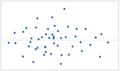
If the assumptions are met, the residuals will be randomly scattered around the center line of zero, with no obvious pattern. The residuals will look like an unstructured cloud of points, centered at zero.

If there is a non-random pattern, the nature of the pattern can pinpoint potential issues with the model.
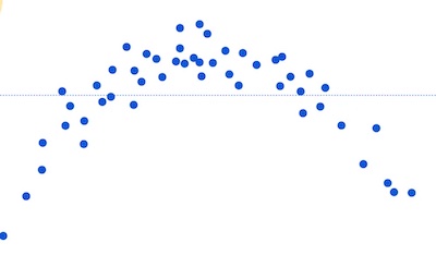
For example, if curvature is present in the residuals, then it is likely that there is curvature in the relationship between the response and the predictor that is not explained by our model. A linear model does not adequately describe the relationship between the predictor and the response.

In this example, the linear model systematically over-predicts some values (the residuals are negative), and under-predict others (the residuals are positive).
Diagnostic plots can help detect whether these assumptions are satisfied. Scatterplots of dependent versus and independent variables are useful for detecting nonlinear relationships, while residual plots are useful for detecting violations of homoskedasticity and independence of errors.
User Contributed Comments 1
| User | Comment |
|---|---|
| alejandroc | Same as univariable, plus multicollinearity. |

Your review questions and global ranking system were so helpful.

Lina
My Own Flashcard
No flashcard found. Add a private flashcard for the subject.
Add