- CFA Exams
- 2024 Level I
- Topic 1. Quantitative Methods
- Learning Module 3. Probability Concepts
- Subject 6. Expected Value (Mean), Variance, and Conditional Measures of Expected Value and Variance
Why should I choose AnalystNotes?
Simply put: AnalystNotes offers the best value and the best product available to help you pass your exams.
Subject 6. Expected Value (Mean), Variance, and Conditional Measures of Expected Value and Variance PDF Download
The expected value of a random variable is its probability-weighted average of the possible outcomes. When combined with probability, the expected value simply factors in the relative chances of each event occurring, in order to determine the overall result. The more probable outcomes will have a greater weighting in the overall calculation.E(X) = P(x1) x1 + P(x2) x2 + ... + P(xn) xn σ2(X) = E{[X - E(X)]2}
X = revenue, F = favorable weather, M = moderate weather, U = unfavorable weather, the formula becomes:
E(X) = E (X|F) x P(F) + E (X|M) x P(M) + E(X|U) x P(U)
E (X|F) = Expected value (Revenue | Favorable weather) = 200,000, because if the weather is favorable, the revenue will be $200,000.
Similarly, E (X|M) = 80,000 and E(X|U) = 0.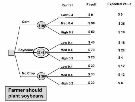
For a random variable X, the expected value of X is denoted E(X).
In investment analysis, forecasts are frequently made using expected value, for example, the expected value of earnings per share, dividend per share, rate of return, etc. It represents the central value of all possible outcomes.
Example
The organizers of an outdoor event know that the success of the event depends on the weather. It costs $50,000 to stage the event. If the weather is favorable, the organizers will take in $200,000. If the weather is moderate, the organizers will take in $80,000. If the weather is unfavorable, the organizers will be forced to abandon the event, and thus take in $0. The weather bureau forecasts that the chances of favorable, moderate and unfavorable weather are 20%, 30% and 50% respectively. Should the organizers go ahead and stage the event?
We can use expected value to work out what revenue the organizers can expect to generate. Once we have this number, we can compare it with the cost of the event, $50,000, to assess whether the venture is likely to be profitable.
Using the expected value formula, we will multiply each amount by its probability, and add the answers. E(X) = 200,000 x 0.2 + 80,000 x 0.3 + 0 x 0.5 = 40,000 + 24,000 + 0 = $64,000
Thus, the organizers can expect to take in $64,000. Since it costs $50,000 to stage the event, this translates to a profit of $14,000, so they should certainly go ahead with the venture.
It's important to realize that none of the outcomes actually produces an amount of $64,000. This is simply the weighted average of all possible outcomes. Although there is a 50% chance of a loss the big profit that will be made the remaining 50% of the time more than offsets this and creates an overall expected profit.
However, with a one-off concert, there is a major risk involved, particularly in the event of unfavorable weather. An easier way to interpret expected value is as follows: If a number of such concerts were held, the organizers can expect to achieve a profit of $14,000 for each concert. So expected values actually make more sense when viewed over the long run.
The variance of a random variable is the expected value (the probability-weighted average) of squared deviations from the random variable's expected value.
Variance is a number greater than or equal to 0.
- If it is 0, there is no dispersion or risk. The outcome is certain.
- Variance greater than 0 indicates dispersion of outcomes.
- Increasing variance indicates increasing dispersion, if all other factors are equal.
- Variance of X is a quantity in the squared units of X; it is difficult to interpret this variance.
The standard deviation is the positive square root of variance.
Variance and standard deviation measure the dispersion of possible outcomes around the expected value of the random variable. If all other factors are equal, increasing variance or standard deviation indicates increasing dispersion of the possible outcomes.
In the example above, we calculated the expected value of revenue to be $64,000. This was before we subtracted the costs. To calculate the variance of the organizers' revenue, we simply take each value, subtract 64,000, square the answer, multiply by the relevant probability in each case, and add.
Var (X) = [200,000 - 64,000]2 x 0.2 + [80,000 - 64,000]2 x 0.3 + [0 - 64,000]2 x 0.5 = 5824000000
The standard deviation is the square root of this number. So, SD(X) = 76,315.13611.
These numbers are often large, particularly if your original data comprises large numbers, as is the case here. Because the calculations for variance and standard deviation yield big numbers, we can conclude that the values in the data set are extremely variable and scattered fairly far away from the expected value.
Parallel to the total probability rule for stating unconditional probabilities in terms of conditional probabilities, total probability rule for expected value states (unconditional) expected values in terms of conditional expected values.
- E(X) = E(X|S)P(S) + E(X|SC)P(SC)
- E(X) = E(X|S1)P(S1) + E(X|S2)P(S2) + ... + E(X|Sn)P(Sn)
(where S1, S2, ..., Sn are mutually exclusive and exhaustive scenarios or events.)
The general case, equation 2, states that the expected value of X equals the expected value of X given Scenario 1, E(X|S1), times the probability of Scenario 1, P(S1), plus the expected value of X given Scenario 2, E(X|S2), times the probability of Scenario 2, P(S2), and so on.
In investments, we make use of any relevant information available in making our forecast. When we refine our expectations or forecasts, we are typically making adjustments based on new information or events; in these cases we are using conditional expected values. The expected value of a random variable X given an event or scenario S is denoted E(X|S).
Relating the formula to the example above and using the following notation:
X = revenue, F = favorable weather, M = moderate weather, U = unfavorable weather, the formula becomes:
E(X) = E (X|F) x P(F) + E (X|M) x P(M) + E(X|U) x P(U)
Note that the right-hand side has three terms because there are three possible weather scenarios.
The E terms on the right are calculated as follows:
E (X|F) = Expected value (Revenue | Favorable weather) = 200,000, because if the weather is favorable, the revenue will be $200,000.
Similarly, E (X|M) = 80,000 and E(X|U) = 0.
So, E(X) = 200,000 x 0.2 + 80,000 x 0.3 + 0 x 0.5 = 40,000 + 24,000 + 0 = 64,000.
This is the same answer that we calculated before; the formula above is just another way of carrying out the same calculation.
Note that had there been ten different weather scenarios, the right-hand side would contain ten different terms. The key information is that the different weather scenarios are both mutually exclusive and exhaustive.
Probability Tree
Probability trees are useful for calculating combined probabilities for sequences of events. It helps you to map out the probabilities of many possibilities graphically, without the use of complicated probability formulas.
A probability tree has two main parts: the branches and the ends(sometimes called leaves). The probability of each branch is generally written on the branches, while the outcome is written on the ends of the branches. In general you multiply along the branches and add probabilities down the columns (up to 1).
Example
Suppose a farmer must decide what to do with his land for the next growing season. He can choose to plant corn or soybeans or to not plant anything at all. If he plants nothing at all, the government farm subsidy will pay him $30 per acre.
If the farmer decides to plant corn or soybeans on his land, there is some risk involved. The yield per acre depends on the amount of rainfall. Too much rain or too little rain will give poorer results than the right amount of rainfall. There is a 40 percent probability that the rainfall will be low; there is a 40 percent probability that the rainfall will be medium; and there is a 20 percent chance that the rainfall will be high.
If the farmer decides to plant corn, the yield per acre will be $0, $90, and $50, respectively, if the rainfall is low, medium, or high. If the farmer decides to plant soybeans, the yield per acre will be $40, $70, and $20, respectively, for low, medium, and high amounts of rainfall.
As shown in the figure, the decision to be made is whether the farmer should plant corn, soybeans, or nothing at all. There are three lines coming out of the decision box to indicate the three choices. Each choice leads to a probabilistic occurrence - how much rainfall will occur.
Each probabilistic occurrence has three possible outcomes - low, medium, or high amounts of rainfall. For each of these events there is an associated payoff. The payoff amount multiplied by the probability of that event occurring is the expected value of each occurrence.
In order to evaluate the decisions, we must add the expected value of each event associated with each decision to get the expected value for each decision. For corn, low rainfall means that no money will be made from the crop. For medium rainfall there is a 40 percent chance and a $90 yield, giving an expected value of $36. For high rainfall there is not as much yield per acre at $50 and there is a 20 percent probability of that occurring. The expected value for high rainfall is thus $10 per acre. Adding the expected values for the events gives us the expected value for the decision. This is $46 per acre.
Using the same calculation for the soybeans and for not planting at all, we see that of the three decisions, planting soybeans has the greatest yield.
User Contributed Comments 7
| User | Comment |
|---|---|
| JGoff | SS2 certainly starts you off :) |
| akif | These are common sense topics which are explained in detail-- i think reeding this in detail is waisting time-- |
| johntan1979 | Someone's waist is growing reeds |
| Shaan23 | Waste of time is writing about this being a waste of time... Im ok with wasting time thats why I wrote this. |
| nishikori | @JGoff SS2 is ancient bro |
| unknown | weeds* |
| khalifa92 | similar terms but different concepts, not a waste of time. |

I was very pleased with your notes and question bank. I especially like the mock exams because it helped to pull everything together.

Martin Rockenfeldt
My Own Flashcard
No flashcard found. Add a private flashcard for the subject.
Add