- CFA Exams
- 2026 Level I
- Topic 1. Quantitative Methods
- Learning Module 8. Hypothesis Testing
- Subject 8. Tests Concerning Differences between Means with Independent Samples
Why should I choose AnalystNotes?
AnalystNotes specializes in helping candidates pass. Period.
Subject 8. Tests Concerning Differences between Means with Independent Samples PDF Download
In practice, analysts often want to know whether the means of two populations are equal or whether one is larger than the other.
If it is reasonable to believe that the samples are from populations at least approximately normally distributed and that the samples are also independent of each other, whether a mean value differs between the two populations can be tested. The test procedure is the same as before. There are just a couple of modifications that need to be made.
As mentioned previously, the null hypothesis involves an equal sign. So, in this situation, the null hypothesis would be that the two unknown population means are equal. The alternative hypothesis would involve one of >, < or ≠.
The rest of the testing procedure is the same, but the test statistic is different. It's now time to look at what formula should be used. Be warned, though, that the formulae in this section are horrific.
The test statistic to be used in this section is a t-value, but it varies based on the assumptions. The assumption has been made throughout that the population means are normally distributed.
1. Test statistic for a test of the difference between two population means (normally distributed populations, population variances unknown but assumed equal):
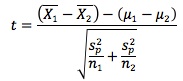
where sp2 = [(n1 - 1)s12 + (n2 - 1)s22] / (n1 + n2 - 2) is a pooled estimator of the common variance. The number of degrees of freedom is n1 + n2 - 2. Normally, the degrees of freedom are given by n - 1, but here there are two samples. Combine the sample sizes and then subtract 1 for each sample, or 2 in total. This gives n1 + n2 - 2 as the degrees of freedom.
2. Test statistic for a test of the difference between two population means (normally distributed populations, unequal and unknown population variances):
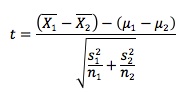
where tables are used to show the t-distribution using "modified" degrees of freedom computed with the formula:
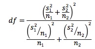
A practical tip is to compute the t-statistic before computing the degrees of freedom. Whether the t-statistic is significant will sometimes be obvious.
Example
From a class of Science students, a sample of 36 is drawn; the mean grade is found to be 62% with a standard deviation of 10. From a class of Arts students, a sample of 49 is drawn; the mean grade is found to be 59% with a standard deviation of 9.6. Assuming that the grades in both classes have a normal distribution, and that the population variances are equal, test at the 5% level for a statistically significant difference in the mean grades of the two classes.
Note that since the sample standard deviations are 10 and 9.6 respectively, the assumption that the population variances are equal seems valid. Had there been a big discrepancy in the sample values, the assumption of equality of population variances would have carried less weight.
"1" will be used to represent the Science students and "2" to represent the Arts students.
Step 1: State the hypotheses.
You are testing for differences in the population means μ1 and μ2. Since the question does not specify a direction, a two-sided test is appropriate. The hypotheses are therefore:
H0: μ1 - μ2 = 0
Ha: μ1 - μ2 ≠ 0
Step 2: Identify the test statistic and its probability distribution.
The appropriate test statistic is the one that assumes equal variances. It is the t-value (discussed earlier).
Step 3: Specify the significance level.
You are told to test at the 5% level, so α = 0.05.
Step 4: State the decision rule.
This is a two-sided test, so you need to split your area equally between both tails. You thus have 2.5% of area in each. The total degrees of freedom are: n1 + n2 - 2 = 36 + 49 - 2 = 83. Your tables don't have 83 degrees of freedom, so use 80, which is the closest value to 83. From the t-table, the critical values are therefore -1.99 and 1.99.
The value above determines your decision. If your test statistic lies to the left of -1.99 or to the right of 1.99, you will reject H0; otherwise, you will not reject H0.
You might notice that your critical values of -1.99 and 1.99 are very close to the corresponding z-values of -1.96 and 1.96. This is because, as explained earlier, as the degrees of freedom increase, the t-values approach the z-values. Since 83 degrees of freedom is a large number, the t-graph here closely resembles a z-graph.
Step 5: Collect the data in the sample and calculate the necessary value(s) using the sample data.
The question gives you the necessary sample values: x-bar1 = 62, x-bar2= 59, s1 = 10, s2 = 9.6, n1 = 36 and n2 = 49.
Recall the formula from earlier: s2p = [35 x 100 + 48 x 92.16] / 83 = 95.466. Now you can substitute into the test statistic: = (62 - 59 - 0) /
 = 1.3988.
The t-value of 1.3988 is now compared with your critical values of -1.99 and 1.99.
Step 6: Make a decision regarding the hypotheses.
Since the value of the test statistic is less extreme (i.e., closer to zero) than the positive critical value, the test statistic falls in the acceptance region. You would thus not reject H0 at the 5% significance level.
You can now conclude that the difference in the average marks of Science and Arts students is not significant when testing at the 5% level.
Note:
- Had you used a p-value approach here, you would have obtained a p-value between 0.1 and 0.2 (closer to 0.2). You can check this for yourself as an exercise. You cannot obtain the p-value exactly from t-tables. Because the value is larger than 0.05, you would not reject H0, so your results are consistent with those above.
- Had you made Science population 2 and Arts population 1, your test statistic would have worked out to be -1.3988, but this would have made no difference in your conclusion, since the test is two-sided. It is better, however, to be guided by the question in this regard.
User Contributed Comments 6
| User | Comment |
|---|---|
| Stoner | 16 observations. 3 independent variables on a multiple regression. When testing for significance using the output from the regression, how many d/f? n-k-1? or n-1? or something else? Please advise. |
| roli79 | I just went through this stuff last night. For multiple regression: df = n-(k+1) n = sample size k = number of parameters being estimated the + 1 accounts for the intercept. df = 16-(3+1) df = 12 I am pretty confident in that answer. If anyone else disagrees please post. This is the wrong los to ask this question, though. |
| whiteknight | why should we use t-statistics in case both the population variance is known ? any comments... |
| achu | population variance is unknown here. |
| epizi | Yea but here you are interested in the equality of the population variance to know which steps to follow.If it wasn't equal, you were to calculated the degree of freedom using the most complex fomular above |
| cschulz316 | what's the deal with that super complicated "modified" degrees of freedom? |

Your review questions and global ranking system were so helpful.

Lina
My Own Flashcard
No flashcard found. Add a private flashcard for the subject.
Add