- CFA Exams
- 2026 Level II
- Topic 1. Quantitative Methods
- Learning Module 7. Big Data Projects
- Subject 4. Model Training
Why should I choose AnalystNotes?
Simply put: AnalystNotes offers the best value and the best product available to help you pass your exams.
Subject 4. Model Training PDF Download
The purpose of model training is to generalize well. The model should neither underfit nor overfit.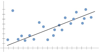
- Positive (P): Observation is positive (for example: is an apple).
- Negative (N): Observation is not positive (for example: is not an apple).
- True Positive (TP): Observation is positive, and is predicted to be positive.
- False Negative (FN): Observation is positive, but is predicted negative. This is Type 2 Error.
- True Negative (TN): Observation is negative, and is predicted to be negative.
- False Positive (FP): Observation is negative, but is predicted positive. This is Type 1 Error.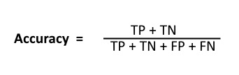
The line below fits within the trend well. It could give a very likely prediction for the new input. In terms of machine learning, the outputs are expected to follow the trend seen in the training set.
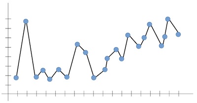
The line below looks good? Yes. But it is not reliable, because it does not capture the dominant trend that we can all see (positively increasing, in our case). It can't predict a likely output for an input that it has never seen before.
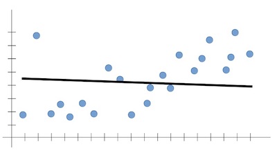
If the model does not learn enough patterns from the training data, it is called underfitting. It results in low generalization and unreliable predictions.
In high bias, the model might not have enough flexibility in terms of line fitting, resulting in a simplistic line that does not generalize well.
Depending on the model at hand, a performance that lies between overfitting and underfitting is more desirable. This trade-off is the most integral aspect of ML model training. ML models fulfill their purpose when they generalize well. Generalization is bound by the two undesirable outcomes - high bias and high variance.
Model fitting errors are caused by a few factors.
- Underfitting can be a result of small datasets or small number of features.
- Overfitting can be caused by large number of features.
The model training process is typically the same for structured and unstructured data.
There are three tasks of model training.
Method Selection
Method selection is governed by the following factors:
- Supervised learning or unsupervised learning. There are supervised selection algorithms which identify the relevant features for best achieving the goal of the supervised model (e.g. a classification or a regression problem) and they rely on the availability of labelled data. For unlabeled data, a number of unsupervised selection methods have been developed which score all data dimensions based on various criteria, such as their variance, their entropy, their ability to preserve local similarity, etc.
- The type of data (numerical, continuous, or categorical; text data; image data; speech data; etc).
- The size of dataset. It is the combination of number of instances and number of features. For example, NNs work well on datasets with large number of instances while SVMs work well on datasets with large number of features.
Once a method is selected, a few tasks may be required before model training begins:
- Make a few method-related decisions (e.g. hyperparameters)
- Split the master dataset into three subsets for supervised learning.
- Deal with class imbalance problem if needed. (oversampling, undersampling)
Performance Evaluation
There are a few techniques discussed in the reading to measure model performance.
Error Analysis
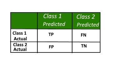
A confusion matrix is a summary of prediction results on a classification problem.The number of correct and incorrect predictions are summarized with count values and broken down by each class. This is the key to the confusion matrix. The confusion matrix shows the ways in which your classification model is confused when it makes predictions.
It gives us insight not only into the errors being made by a classifier but more importantly the types of errors that are being made.
Definitions:
- Positive (P): Observation is positive (for example: is an apple).
- Negative (N): Observation is not positive (for example: is not an apple).
- True Positive (TP): Observation is positive, and is predicted to be positive.
- False Negative (FN): Observation is positive, but is predicted negative. This is Type 2 Error.
- True Negative (TN): Observation is negative, and is predicted to be negative.
- False Positive (FP): Observation is negative, but is predicted positive. This is Type 1 Error.
Accuracy is given by the relation:
However, there are problems with accuracy. It assumes equal costs for both kinds of errors. A 99% accuracy can be excellent, good, mediocre, poor or terrible depending upon the problem.
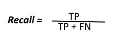
Recall can be defined as the ratio of the total number of correctly classified positive examples divide to the total number of positive examples. High Recall indicates the class is correctly recognized (small number of FN).
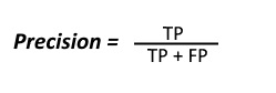
To get the value of precision we divide the total number of correctly classified positive examples by the total number of predicted positive examples. High Precision indicates an example labeled as positive is indeed positive (small number of FP).
High recall, low precision: This means that most of the positive examples are correctly recognized (low FN) but there are a lot of false positives.
Low recall, high precision: This shows that we miss a lot of positive examples (high FN) but those we predict as positive are indeed positive (low FP)
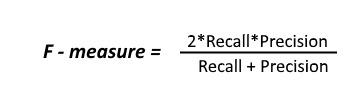
Since we have two measures (Precision and Recall) it helps to have a measurement that represents both of them. We calculate an F-measure which uses Harmonic Mean in place of Arithmetic Mean as it punishes the extreme values more.
The F-Measure will always be nearer to the smaller value of Precision or Recall.
Receiver Operating Characteristics
To carry out receiver operating characteristics (ROC) analysis, ROC curves and area under the curve (AUC) of various models are calculated and compared. The more convex the ROC curve and the higher the AUC, the better the model performance.
Test A is superior to test B because at all cut-offs the true positive rate is higher and the false positive rate is lower than for test B. The area under the curve for test A is larger than the area under the curve for test B.
Root Mean Square Error (RMSE)
This measure is for continuous data prediction. The smaller the measure, the better the model performance.
Tuning
Tuning models means tuning hyperparameters.Model parameters are learned attributes that define individual models. They can be learned directly from the training data. Examples are regression coefficients, decision tree split locations.
Hyperparameters express "higher-level" structural settings for algorithms. They are decided before fitting the model because they can't be learned from the data. Examples are strength of the penalty used in regularized regression, or the number of trees to include in a random forest.
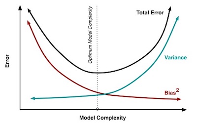
When a model is less complex, it ignores relevant information, and error due to bias is high (underfitting). As the model becomes more complex, error due to bias decreases.
On the other hand, when a model is less complex, error due to variance is low. Error due to variance increases as complexity increases. Generally, a complex or flexible model will tend to have high variance due to overfitting but lower bias.
Overall model error is a function of error due to bias plus error due to variance. The ideal model minimizes error from each.
User Contributed Comments 0
You need to log in first to add your comment.

I just wanted to share the good news that I passed CFA Level I!!! Thank you for your help - I think the online question bank helped cut the clutter and made a positive difference.

Edward Liu
My Own Flashcard
No flashcard found. Add a private flashcard for the subject.
Add