Formal Definition

What is the most I can lose on this investment?

Volatility is often used as a popular measure of risk. The main problem with volatility is that it does not address the direction of price movement. The focus in VaR is downside risk and potential losses. Its use in banks reflects their fear of a liquidity crisis, where a low-probability catastrophic occurrence creates a loss that wipes out the capital and creates a client exodus.

Value at risk (VaR) measures the potential loss in value of a risky asset or portfolio over a defined period for a given confidence interval. It has three components: a time period, a confidence level, and a minimum loss amount (or loss percentage).

For example, if the VaR on an asset is $100 million at a one-week, 95% confidence level, there is a 5% chance that the value of the asset will drop more than $ 100 million over any given week.

The choice of minimum loss magnitude, the confidence level, and the time horizon is subjective.

The VaR can be specified for an individual asset, a portfolio of assets, or for an entire firm.

Estimating VaR

VaR requires the decomposition of portfolio performance into risk factors.

There is no single right way of estimating VaR. Three methods of estimating VaR are presented here.

The Parametric Method

If returns are assumed to be normally distributed, we can use the mean and standard deviation to plot a normal distribution curve. We then automatically know where the 5% and 1% lie on the curve.

• 95% of confidence level: 1.65 standard deviation
• 99% of confidence level: 2.33 standard deviation

Assume that you are assessing the VaR for a single asset, where the potential values are normally distributed with a mean of $100 million and an annual standard deviation of $10 million. With 95% confidence, you can say that the value of this asset will not drop below $80 million (two standard deviations below the mean) or rise about $120 million (two standard deviations above the mean) over the next year.

When working with portfolios of assets, the method will get complicated because of the fact that the assets in the portfolio often move together.

We can convert one horizon or confidence level to another.

The Historical Simulation

In this approach, the VaR for a portfolio is estimated by creating a hypothetical time series of returns on that portfolio, obtained by running the portfolio through actual historical data and computing the changes that would have occurred in each period.

It then simply re-organizes actual historical returns, putting them in order from worst to best. For example, a 5% VaR will be the fifth percentile on the array (meaning that 95% of the outcomes are better than this outcome).

Example

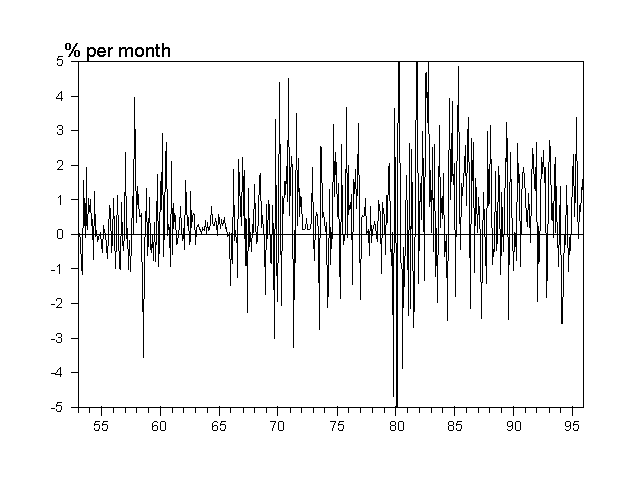
We obtain monthly returns on medium-term bonds from 1953 to 1995.

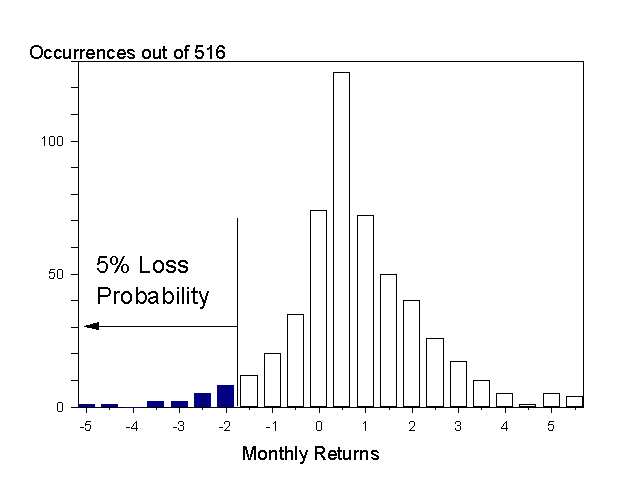
Returns ranged from a low of -6.5% to a high of +12.0%. Now construct regularly spaced "buckets" going from the lowest to the highest number and count how many observations fall into each bucket. For instance, there is one observation below -5%. There is another observation between -5% and -4.5%. And so on. By doing this, you will construct a probability distribution for the monthly returns, which counts how many occurrences have been observed in the past for a particular range.

For each return, you can then compute the probability of observing a lower return. Pick a confidence level, say 95%. For this confidence level, you can find a point on the graph with a 5% probability of finding a lower return. This number is -1.7%; all occurrences of returns less than -1.7% add up to 5% of the total number of months, or 26 out of 516 months.

You are now ready to compute the VaR of a $100 million portfolio. There is only a 5% chance that the portfolio will fall by more than $100 million times -1.7%, or $1.7 million.

There are no underlying assumptions of normality. The approach is based on the assumption of history repeating itself. In a market where risks are volatile and structural shifts occur at regular intervals, this assumption is difficult to sustain.

The Monte Carlo Simulation

The third method involves developing a model for future portfolio returns and running multiple hypothetical trials through the model. A Monte Carlo simulation refers to any method that randomly generates trials but by itself does not tell us anything about the underlying methodology.

• It avoids the complexity inherent in the parametric method when a portfolio has a large number of assets.
• It is not constrained by the assumption of normal distributions. For example, it can accommodate portfolios with embedded options.

The Monte Carlo simulation is complex, but has the advantage of allowing users to tailor ideas about future patterns that depart from historical patterns.

Advantages and Limitations of VaR

The advantages of VaR include the following:

• It is a simple concept, and relatively easy to understand.
• It is easily communicated, capturing a great deal of information in a single number.
• It can be useful in comparing risks across asset classes, portfolios, and trading units.
• It facilitates capital allocation decisions.
• It can be used for performance evaluation.
• It can be verified by using backtesting.
• It is widely accepted by regulators.

The primary limitations of VaR are:

• It is a subjective measure and is highly sensitive to numerous discretionary choices made in the course of computation.
• It can underestimate the frequency of extreme events.
• It fails to account for a lack of liquidity.
• It is sensitive to correlation risk.
• It is vulnerable to trending or volatility regimes.
• It is often misunderstood as a worst-case scenario.
• It can oversimplify the picture of risk.
• It focuses heavily on the left tail.

Extensions of VaR

There are numerous variations and extensions of VaR that can provide additional useful information.

Conditional VaR is the average loss conditional on exceeding the VaR cutoff.

Incremental VaR measures the change in portfolio VaR as a result of adding or deleting a position from the portfolio or if a position size is changed relative to the remaining positions. It is the difference between the "before" and "after" VaR.

Marginal VaR measures the change in portfolio VaR given a small change in the portfolio position. In a diversified portfolio, MVaRs can be summed to determine the contribution of each asset to the overall VaR.

Ex ante tracking error (relative VaR) measures the degree to which the performance of a given investment portfolio might deviate from its benchmark.